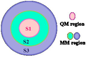
ARAZ

ARAZ serves as an interface that seamlessly integrates the functionality of the ORCA and AMBER program packages for conducting QM/MM calculations [1]. This Linux bash script amalgamates various subprograms, all developed using the Python programming language. To utilize ARAZ effectively, it is essential to have the ORCA, AMBERand Multiwfn programs installed on your machine. These programs collectively handle the QM aspects, MM computations, and the determination of the charge of the QM system. The calculated charge is then automatically updated in the topology file of the entire system during each iteration of the calculations.

ARAZ employs electrostatic embedding to account for environmental effects and calculates the QM/MM energy using the subtractive approach [2]. The system is partitioned into three distinct components: S1, which undergoes treatment using a QM or DFT method; S2, managed by an MM method and subject to optimization throughout the calculations; and finally, S3, treated by an MM method but held fixed during the computation. These components are illustrated in Figure 1.

Figure 1. Illustration of the typical system utilized in QM/MM calculations with ARAZ.

To initiate QM/MM calculations with ARAZ, follow the procedure below:

1. Ensure your structure is equilibrated. Create a PDB file of the equilibrated structure, including point charges in the last column.

1.1 Set up the protein and parameterize hetero groups (cf. link1 and link2 pages). For organic reaction systems, parametrize only the reacting molecules.

1.2 Protonate and solvate the structure following points 1 and 2 on this page.

1.3 Equilibrate the solvated structure with the sander or pmemd module of AMBER as follows:

To equilibrate a periodic system, typically an octahedral box of water molecules, run MD simulations as shown below. Replace 'sander' with 'pmemd' if you have installed this module. Also, replace '28' with the maximum number of CPU cores on your machine.

mpirun -bind-to core -np 28 sander.MPI -O -i sander.in00H -o sander.out00H -p prmtop -c prmcrd -r mdrest00H -ref prmcrd

mpirun -bind-to core -np 28 sander.MPI -O -i sander.in00 -o sander.out00 -p prmtop -c mdrest00H -r mdrest00 -ref prmcrd

mpirun -bind-to core -np 28 sander.MPI -O -i sander.in0 -o sander.out0 -p prmtop -c mdrest00 -r mdrest0 -ref prmcrd

mpirun -bind-to core -np 28 sander.MPI -O -i sander.in1 -o sander.out1 -p prmtop -c mdrest0 -r mdrest1 -ref prmcrd

mpirun -bind-to core -np 28 sander.MPI -O -i sander.in2 -o sander.out2 -p prmtop -c mdrest1 -r mdrest2 -ref prmcrd

In the above lines, replace sander with pmemd if you have installed this module. Also, replace '28' with the maximum number of CPU cores of your machine. The contents of the sander.in files are provided below:

The sander.in00H file.

Minimization without shake, All hydrogen atoms

&cntrl

irest=0,ntx=1,

nstlim=0,dt=0.0005,

imin=1,maxcyc=1000,drms=0.001,

temp0=300.0,ntt=3,gamma_ln=2.0,

ntc=1,ntf=1,

nsnb=40,cut=8.0,dielc=1.0,

ntpr=100,ntwx=0,ntwv=0,ntwe=0,

ntb=1,ntp=0,taup=0.2,

ipol=0,igb=0,

ncyc=10,ntmin=1,dx0=0.01,

ntr=1,restraint_wt=1000,

restraintmask=" !@H="

&end

The sander.in00 file

Minimization without shake.

&cntrl

irest=0,ntx=1,

nstlim=0,dt=0.0005,

imin=1,maxcyc=1000,drms=0.001,

temp0=300.0,ntt=3,gamma_ln=2.0,

ntc=1,ntf=1,

nsnb=40,cut=8.0,dielc=1.0,

ntpr=100,ntwx=0,ntwv=0,ntwe=0,

ntb=1,ntp=0,taup=0.2,

ipol=0,igb=0,

ncyc=10,ntmin=1,dx0=0.01,

&end

The sander.in0 file

10 ps MD simulation without shake

&cntrl

irest=0,ntx=1,

nstlim=20000,dt=0.0005,

imin=0,maxcyc=100,drms=0.001,

temp0=300.0,ntt=3,gamma_ln=2.0,

ntc=1,ntf=1,

nsnb=40,cut=8.0,dielc=1.0,

ntpr=1000,ntwx=0,ntwv=0,ntwe=0,

ntb=1,ntp=0,taup=0.2,

ipol=0,igb=0,

ncyc=10,ntmin=1,dx0=0.01,

&end

The sander.in1 file

1 ns equilibration with shake and constant volume

&cntrl

irest=1,ntx=5,

nstlim=500000,dt=0.002,

temp0=300.0,ntt=3,gamma_ln=2.0,

ntc=2,ntf=2,

nsnb=15,cut=8.0,dielc=1.0,

ntpr=1000,ntwx=0,ntwv=0,ntwe=0,

ntb=1,ntp=0,taup=0.2,

ipol=0,igb=0,

&end

The sander.in2 file

1 ns simulated annealing at constant pressure

&cntrl

irest=1,ntx=5,

nstlim=500000,dt=0.002,

temp0=300.0,ntt=3,gamma_ln=2.0,

ntc=2,ntf=2,

nsnb=15,cut=8.0,dielc=1.0,

ntpr=1000,ntwx=0,ntwv=0,ntwe=0,

ntb=2,ntp=1,pres0=1.0,taup=1.0,

ipol=0,igb=0,

nmropt=1,

&end

&wt type='TEMP0',istep1= 0,istep2=160000,value1=370.00,value2=370.00 &end

&wt type='TEMP0',istep1=160001,istep2=500000,value1=370.00,value2= 0.00 &end

&wt type='TAUTP',istep1= 0,istep2=200000,value1= 0.20,value2= 0.20 &end

&wt type='TAUTP',istep1=200001,istep2=320000,value1= 1.00,value2= 1.00 &end

&wt type='TAUTP',istep1=320001,istep2=400000,value1= 0.50,value2= 0.50 &end

&wt type='TAUTP',istep1=400001,istep2=500000,value1= 0.05,value2= 0.05 &end

&wt type='END' &end

To equilibrate a non-periodic system, typically a PDB structure with organic solvents from Packmol, run MD simulations as described in point 4.2 on this page.

The final coordinate of the MD simulations of the octahedral box of water molecules is stored in the mdrest2 file, and we have to convert it to a PDB file.

1.4 Convert the equilibrated system to a PDB file.

1.4.1 Execute the following command. It wraps the water molecules in the mdrest2 file into another file called mdrest2-wrap.

cpptraj prmtop ptraj.in

The contents of the ptraj.in file are as follows:

where "1" is the residue number of the central residue in the pdbout file.

The ptraj.in file

trajin mdrest2

trajout mdrest2-wrap restart

image origin center familiar com :1

You can obtain the residue number of the central residue by running the command "cap center" in changepdb. A graphical program such as RasMol can also be used to find the central residue.

1.5 Convert the mdrest2-wrap file to PDB format using topologyanalyser.

topologyanalyser <<EOF

prmtop

mdrest2-wrap

araz-in.pdb

EOF

Now you can use the araz-in.pdb file in the following steps. Note that if you already have the final structure from the simulations of the system generated by Packmol and stored in the equil.pdb file, there is no need to perform the above conversion steps for the mdrest2-wrap file. To do this, you need to use topologyanalyser to generate a pdb file that has point charges in the last column.

2. Describe the QM system in a text file

You will need a text file describing the QM system (by default, named 's1' in our programs). Below is an example 's1' file. The first line serves as the project title. Lines beginning with 'QM:' denote the atomic numbers of atoms from the initial PDB file that should be included in the QM system. For example, '1316-1319' implies that atoms 1316, 1317, 1318, and 1319 will be part of the QM system. You can add comments to each line after '!' if desired; the program (arazprep) will ignore text following '!' on a line. Lines starting with 'CL:' identify CL junctions. Finally, lines starting with 'X:' identify the neighbors of each CL atom that are covalently bonded to it in the QM region (refer to Scheme 1). Feel free to adjust the comments and descriptions based on the specifics of your system.

A sample s1 file.

Title: 05-Rieske RED, AH1, CH=-1, u=0

QM: 1316-1319 ! CYM-87

QM: 1340-1349 ! HIN-89

QM: 1586-1589 ! CYM-106

QM: 1620-1630 ! HIE-109

QM: 2313-2316 ! 2FE(III,III), 2S

CL: 1314 1338 1584 1618

X: 1316 1340 1586 1620

Scheme 1: Representation of CL, HL, and X atoms. Atoms from the starting PDB file in the QM and MM systems are depicted in green and blue, respectively.

3. 3. Run the arazprep program as follows or customize it according to your file names.

arazprep <<EOF

araz-in.pdb

6.0

yes

-1

EOF

3.1 Choose the starting PDB file.

3.2 If you are working with a protein, choose option 1 for TER; otherwise, choose option 2 for TER.

3.3 Enter the name of the S1 file, which describes the QM system.

3.4 Enter the title of your project.

3.5 Enter the most accurate CL-HL bond lengths.

3.6 Enter the thickness of S2 around the QM system.

3.7 Enter the level of theory.

3.8 Enter the number of CPU cores for parallel calculations.

3.9 Enter the charge of the QM system.

3.10 Enter the multiplicity of the QM region.

The program creates the following files, each described in Table 1.

Table 1. Files and Their Descriptions Created by the arazprep Program:

File name

Description

1

pdbWithTER.pdb

PDB file of the entire system with TER lines at proper places.

2

tided_up_pdb.tmp

The tidied-up PDB file of the whole QM/MM system.

3

pdb_0_charge.pdb

PDB file of the entire QM/MM system with point charges of the QM system set to zero.

4

qm.pdb

PDB file of the QM system.

5

qmC0.pdb

PDB file of the QM system with atomic partial charges at the last column set to zero. This file is necessary to set the charge of the prmtop1 file to zero in the following steps.

7

energy.in

The sander.in file to calculate the MM energy of the QM system and the MM energy of the whole system.

8

s2_opt.in

The sander.in file to optimize the MM system with AMBER. The belly list is included at the end of the file.

9

HL-Atoms.txt

Atom numbers of the HL atoms in the qm.pdb file.

10

CL-Atoms.txt

Atom numbers of the CL atoms in the starting PDB file.

11

QM-Atoms.txt

Atom numbers of the QM system atoms in the starting PDB file of the entire system. The atomic numbers of the CL atoms are also included in this file.

12

QM-CL-Atoms.txt

Atom numbers of the QM system atoms in the starting PDB file of the entire system. The atomic numbers of the CL atoms are also included in this file.

13

pointcharges.pc

Point charges of the MM system.

14

araz.inp

ORCA input file to perform the QM part of the QM/MM calculations.

4. Create the Topology File of the QM System

4.1 Insert TER between fragments of the qm.pdb file.

pdbanalyser <<EOF

qm.pdb

ter

qm-ter.pdb

EOF

4.2 Extract the fragments of the qm.pdb file, each in a separate file. Example:

grep "CYM" qm-ter.pdb > cym.pdb

grep "HIN" qm-ter.pdb > hin.pdb

grep "HIE" qm-ter.pdb > hie.pdb

4.3 Create parameters for each fragment.

antechamber -i cym.pdb -fi pdb -o cym.in -fo prepi -nc -1 -c bcc -rn CYM -at gaff

antechamber -i hin.pdb -fi pdb -o hin.in -fo prepi -nc -1 -c bcc -rn HIN -at gaff

antechamber -i hie.pdb -fi pdb -o hie.in -fo prepi -nc 0 -c bcc -rn HIE -at gaff

parmchk2 -i cym.in -f prepi -o cym.dat

parmchk2 -i hin.in -f prepi -o hin.dat

parmchk2 -i hie.in -f prepi -o hie.dat

4.4 Run tleap with the tleap-qm.in to create the topology and coordinate files of the QM system with HL junctions (prmtop1 prmcrd1, respectively).

tleap -s -f tleap-qm.in

Here is a sample tleap-qm.in file:

#source leaprc.protein.ff14SB

source leaprc.gaff

#source leaprc.water.tip3p

addPath /home/mehdi/araz-test/Parm/

loadAmberPrep fe3.in

loadAmberPrep su2.in

loadAmberPrep hin.in

loadAmberPrep hie.in

loadAmberPrep cym.in

loadAmberParams fe.dat

loadAmberParams su2.dat

loadAmberParams hin.dat

loadAmberParams hie.dat

loadAmberParams cym.dat

x=loadpdb qm-ter.pdb

saveamberparm x prmtop1 prmcrd1

savepdb x pdbout1

quit

4.5 Make the atomic partial charges of all systems in the prmtop1 equal to zero.

topologyanalyser <<EOF

prmtop1

qmC0.pdb

EOF

5. Create prmtop3, the topology file of the whole system using tleap.

tleap -s -f tleap.in

Here is a sample tleap.in file:

source leaprc.protein.ff14SB

source leaprc.gaff

source leaprc.water.tip3p

addPath /home/mehdi/araz-test/Leap/

loadAmberPrep fe3.in

loadAmberPrep su2.in

loadAmberPrep hin.in

loadAmberParams fe.dat

loadAmberParams su2.dat

loadAmberParams hin2.dat

loadAmberParams hin1.dat

x=loadpdb pdbWithTER.pdb

bond x.92.SG x.108.SG

saveamberparm x prmtop3 prmcrd3

quit

6. Create the topology file of the whole system with charges of the QM system as zero (prmtop2).

topologyanalyser <<EOF

prmtop3

pdb_0_charge.pdb

prmtop2

EOF

3. Run the program as:

araz.free

References

[1] U. Ryde, QM/MM Calculations on Proteins, Methods Enzymol. 577 (2016) 119–158. https://doi.org/10.1016/BS.MIE.2016.05.014.

[2] L. Cao, U. Ryde, On the difference between additive and subtractive QM/MM calculations, Front. Chem. 6 (2018) 359025. https://doi.org/10.3389/FCHEM.2018.00089/BIBTEX.